Measuring Running Power

For exercises such as running and cycling, power output provides an unbiased metric for effort as compared to, for example, speed, irrespective of external conditions, such as wind and terrain.

Power output is a widely used and well-defined metric in cycling. For power based training Functional Threshold Power (FTP), the highest sustainable power output of a cyclist over a period of 60 minutes, is first determined. The power training routine then consists of periods in predefined ‘power zones’ that are based on a cyclist’s FTP. Cycling power is typically measured with strain gauges at the crank.

For running, however, there’s no agreed way to measure power output. Of course, it can be measured with force plates on a treadmill, but it’s not a viable option for running on a track. There are multiple techniques of measuring running power, one of which is Stryd, that estimates power using an accelerometer mounted on top of a foot. Their technology is proprietary, but there is a proposed model for power measurements, External Energy Summation Approach (EESA), that is described by Ron George, and that seem to align well, with the results obtained from the Stryd power meter.

EESA is a comprehensive model that can approximate running power and how it changes over time, accounting for different conditions. Eventually, we would like to implement this model and perform such running power measurements, however, as a first exercise, we will only measure total work done (and hence average power) against external forces on a straight path with a much simpler model.

Hardware-wise we are using Arduino Nano IoT that will measure the acceleration and send it over Bluetooth Low Energy (BLE) to an Android smartphone.

Accessing and sending the IMU data

First, we need a way to record the acceleration. The Arduino Nano IoT has LSM6DS3 IMU (Inertial Measurement Unit) on board, providing acceleration and angular velocity via a library. With the default output data rate of 104 Hz, we can poll the IMU for measurements every 10 milliseconds using this code

#define IMU_POLLING_PERIOD 10
void setup() {
  ...
  if (!IMU.begin()) {
    Serial.println("Failed to initialize IMU!");
    while (true); // halt program
  }
  ...
}

void pollIMU() {
  float aX, aY, aZ;
  float gX, gY, gZ;
  unsigned long time;
  const char * spacer = ", ";

  if (
    IMU.accelerationAvailable()
    && IMU.gyroscopeAvailable()
  ) {
    IMU.readAcceleration(aX, aY, aZ);
    IMU.readGyroscope(gX, gY, gZ);
    time = millis();

    reading = {
      .reading = {
        .time = time,
        .acceleration = {aX, aY, aZ},
        .gyroscope = {gX, gY, gZ}
      }
    };
    ...
  }
}

void loop() {
  ...
  if (currentMillis - lastMillis >= IMU_POLLING_PERIOD) {
    lastMillis = currentMillis;
    pollIMU();
  }
  ...
}

In this code we use the variable reading that is defined as follows

• Firstly, we define a structure to store three components of a vector.
• Secondly, we define a structure to hold time of the reading (the internal clock is used), and two vectors for acceleration and angular velocity.
• Finally, we build a union of this struct with a byte array of the same size (that is needed for serialisation before sending via Bluetooth), which is then filled in with actual data within pollIMU function.

typedef struct{
float x;
float y;
float z;
} vector3d_struct_t;

typedef struct{
unsigned long time;
vector3d_struct_t acceleration;
vector3d_struct_t gyroscope;
} imu_reading_struct_t;

typedef union{
imu_reading_struct_t reading;
uint8_t array[sizeof(imu_reading_struct_t)];
} imu_reading_t;

imu_reading_t reading = {};

In order to collect the readings with the smartphone we will send the data over Bluetooth Low Energy (BLE) using the Arduino BLE library as follows:

• Define a BLE service (the UUID is arbitrary, and is used to filter for BLE devices that provide certain functionality)
• Define a BLE characteristic. This can be thought of as a register, that can hold some value, and allows some actions to be performed by a central device (the smartphone in this case). For our purposes, we define a characteristic of size of our record, that can be read and subscribed for update notification.
• Wait for a central device to connect, and update the characteristic value in pollIMU function while connection is maintained

BLEService powermetreService("1FFF");
BLECharacteristic imuReadingChar("2FFF", BLERead | BLENotify, sizeof(imu_reading_t));

void setup() {
...
if (!BLE.begin()) {
Serial.println("starting BLE failed!");
while (true);
}
Serial.println("BLE started");
BLE.setLocalName("Powermetre");
BLE.setAdvertisedService(powermetreService);
Serial.println(powermetreService.uuid());
powermetreService.addCharacteristic(imuReadingChar);
BLE.addService(powermetreService);
imuReadingChar.writeValue(reading.array, sizeof(reading.array));
BLE.advertise();
Serial.println("BLE setup finished.");
}

void loop(){
BLEDevice central = BLE.central(); // Wait for connection
if(central) {
Serial.print("Central device connected: ");
Serial.println(central.address());
digitalWrite(LED_BUILTIN, HIGH);
while(central.connected()) {
  long currentMillis = millis();
  if (currentMillis - lastMillis >= IMU_POLLING_PERIOD) {
    lastMillis = currentMillis;
    pollIMU();
  }
}
digitalWrite(LED_BUILTIN, LOW);
}
}

The results can now be subscribed for, collected and stored with any BLE capable device. The full Arduino code and the accompanying Android app are available on Github.

Power analysis

Even though we cannot perform measurements done by Stryd straight away, we can still approximate the work done from accelerometer data against external forces, with a few assumptions. Firstly, we assume that we are walking in a straight line; that way we only have to consider forces in one direction. And secondly, we assume that our speed is constant in the duration of a walk.

Work done for a straight path can simply be defined as an integral of a force F over displacement s. F in this case is a force vector in the direction of the walk (work done in two other orthogonal directions is assumed to be zero). By the second law, we know that F=ma, where m is a mass of a body, and a is an acceleration vector in the desired direction. For this experiment we simply measure out the path of 4.5 metres, mount the power metre on the chest, and walk trying to maintain speed. After the recording is done, we can analyse the results in a Jupyter Notebook.

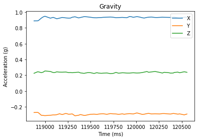
Removing gravity

As a calibration step we estimate and subtract the gravity vector. Even though it is not strictly necessary if we know the exact direction we are walking at, as those vectors are supposed to be orthogonal, we only have the approximate direction (due to imprecise positioning of the sensor on the body).

To estimate it, we take a few seconds of standing still before walking when the only acceleration measured should be the gravity and take the mean average of that.

rps = 100 # records per second
_df = df.iloc[22*rps:25*rps] # hand-picked range
gravity_vector = _df.loc[:,["aX", "aY", "aZ"]].mean()
display(ground_vector.values, np.sqrt((ground_vector**2).sum()))

# array([ 0.93137248, -0.29392049,  0.2339799 ])
# 1.0042860847765203

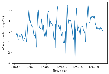
Estimate work done

With the resulting acceleration readings we can estimate how much work has been done. From here on we assume that the direction of the walk is -Z. Remembering our assumption of constant speed and known overall displacement, we calculate the work done and the average power as follows

# Take only the records corresponding to the walk
rps = 100 # records per second
a, b = int(26 * rps), int(35.5 * rps)
sample = acceleration.iloc[a:b]
mass = 85
time = (sample.time - sample.time.min()) / 1000
dtime = (sample.time.max() - sample.time.min()) / 1000 # Total duration of a walk in seconds
# Mean average speed.
vbar = 4.5 / dtime
# Estimate displacement with the constant speed. 
x = [x * vbar for x in time.values]
# Integrate force with respect to displacement 
work = sp.integrate.trapz(y=-sample.aZ.values * mass, x=x)
print(f"Time: {dtime} s.\nSpeed: {vbar} m/s.\nAvg. power: {work / dtime} W.\nWork: {work} J.")

# Time: 5.48 s.
# Speed: 0.8211678832116788 m/s.
# Avg. power: 20.991248881466902 W.
# Work: 115.03204387043863 J.

Validating results

To validate that our results are reasonable, we have also recorded acceleration with a built-in accelerometer of an Android phone. Straight away we can see that even though the exact values are different, the overall pattern is similar. The differences can be partially accounted for by the lower sampling rate of the Android accelerometre.

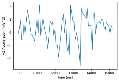
Performing the same calculations on this data yields similar results with only about 1 Watt of difference.

Time: 5.207 s.
Speed: 0.8642212406376033 m/s.
Avg. power: 19.814510206149293 W.
Work: 103.17415464341937 J.

Limitations

Even though the estimate of work with the current approach is reasonable, there are multiple limitations that need to be addressed.

First of all, we try to position the sensor such that -Z axis aligns with the path, but it is not perfect. There does not seem to be an obvious solution to calibrate for walking direction in a similar way we calibrated for the direction of the gravity. This results in the work done being underestimated (since work done in two other orthogonal directions is not exactly zero).

Secondly, this model will not account for turning, as we only consider work to be done along single axis.

Both of this limitations can be mitigated if we employ the EESA model suggested by Ron George. However, it requires the instant velocity to be estimated from acceleration. Where we come to our third limitation, imprecise measurements. Trying to integrate acceleration over time we get increasing velocity, whereas we expect the velocity to come back to zero at the end of the walk.

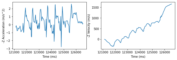
For the same reason (lack of instant velocity measurements), we cannot estimate instant power in a way Stryd does it. Therefore, this needs to be considered as the most important issue, the solution for which is yet to be found (be it some signal processing required, or use of a different sensor).

This is an on-going project, and there more things to come, but for now, we encourage everyone interested to see the current implementation, and try it out for themselves, on Github, that hosts the code for Arduino, Android app, and notebooks with analysis performed (along with some sample data).