Smart Insole Analytics step-by-step

Itching to turn our exercise into data, last year the Fuzzy Labs team embarked upon a project to put sensors in our trainers (sneakers, for Americans out there), and connect our shoes to the Internet of ‘things’ - because that’s what we’re like.

Our ultimate aim is to build an open-source platform for combining AI models with wearable hardware. The prototype hardware is described in a previous blog post - although we’ve since moved to the newer, sleeker Arduino Nano IOT in place of the bulkier ESP32 for a marginally less ugly-looking form factor.

In this article I’ll demonstrate some sample data collected by the device and perform rudimentary time-series analysis, finally rendering the results using the Dash Framework.

All source code and schematics are available here.

Getting a foot-hold

The prototype device consists of three pressure sensors attached to an inexpensive foam insole. The sensors are each sampled every second by a microcontroller and these readings are transmitted to a smartphone over Bluetooth.

We’ll begin by exploring the data in Jupyter. We have a CSV file in which each row has a timestamp (as as ISO-8601 date-time) and a set of sensor readings, like so:

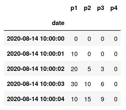
We’ll load this as a time series using Pandas:

import pandas as pd
 pressure_data = pd  \
   .read_csv("../data/sample.csv", index_col=0, parse_dates=[0]) \ 
   .query('date != "NaT"') 

Three things to pay attention to here:

• index_col=0 - this tells Pandas to use the timestamp column as an index.
• parse_dates=[0] - this tells Pandas to parse column 0 as a dates.
• By removing NaT (Not a Time) values we filter out any rows where the date field can’t be read. If the device is behaving itself, then we don’t expect this to happen, however this step is included as good practice in case of future data corruption.

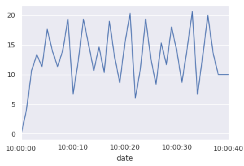
Next, let’s plot the timeseries:

pressure_data.plot()

Each sensor has its own line. The peaks of those lines indicate where maximum pressure is being applied, which is something we can use to count steps and measure cadence.

Step-by-step metrics

Using the pressure sensors, we’d like to calculate two metrics:

• Step count: the total number of footsteps during an exercise
• Cadence: the average number of steps per minute

Step counting

Walking, jogging, running, etc. happen to be repetitive activities. As a result, the graph of pressure over time is more-or-less periodic. We can use the peaks or maxima of this graph to represent steps.

The trouble is, we have multiple pressure sensors, each with their own graph. Naïvely we could pick one of these sensors to use a basis for counting steps, let’s say the first one, which is connected to the heel. Then we’ll count any value within 25% of the maximum pressure as one step.

def count_steps_naive(dataframe):
    column = "p1"
    p_max = dataframe[column].max()
    p_min = dataframe[column].min()
    target_pressure = p_max - 0.25 * (p_max - p_min)
    matching_rows = dataframe[dataframe[column] >= target_pressure]
    return matching_rows[column].count()

With this approach there are a number of problems, but the most significant is that we’re not taking into account all of sensors and furthermore, the sensor readings can be a little bit noisy, which can lead to false-positives while counting steps.

A better method can be found in A comparative study of smart insole on real-world step count (Feng Lin et al, 2015 IEEE Signal Processing in Medicine and Biology Symposium).

The authors first calculate the average pressure across all sensors. We’ll do the same, calculating the mean with axis=1 so that we get a time series with one column that represents the average of all sensors for each point in time.

p_avg = pressure_data.mean(axis=1)

Next they calculate the rate of change, or differential of average pressure as it’s called in the paper:

p_diff = p_avg.diff()

Finally, the authors choose two threshold parameters, which are discovered by experimentation. In the paper, they use γ and Γ, but we’ll just call these parameters low_threshold and high_threshold. Here’s the enhanced step counting function:

def count_steps(dataframe, low_threshold = 0, high_threshold = 4):
    p_avg = dataframe.mean(axis=1)
    p_diff = p_avg.diff()
    status = 0
    step_count = 0
    for p_diff_t in p_diff:
        if p_diff_t < low_threshold:
            if status == 1:
                step_count += 1
            status = -1
        elif p_diff_t > high_threshold:
            status = 1
    return step_count

Deviating from the paper I’ve used different values for the low and high thresholds due to differences in the measurements range on this hardware.

Note that as we’re only using one insole, we need to multiply the result by 2 to get the true step count using either of these methods.

Cadence

Armed with our step counting function we can go on to implement a common metric used in running, jogging and similar activities, cadence.

Cadence is measured in strides or steps per minute. People of different heights will have different stride lengths, and therefore they will require a different number of steps in order to cover the same distance, so if we’re using cadence to compare two runners, we have to know their height too, but for our purposes we’ll ignore that detail.

To calculate cadence with Pandas we’ll simply invoke the step counter and divide by the exercise duration in seconds:

def calculate_cadence(dataframe):
    duration = (dataframe.index.max() - dataframe.index.min()).seconds
    return count_steps(dataframe) / float(duration)

See https://www.trainingpeaks.com/blog/finding-your-perfect-run-cadence for more discussion on how cadence is used in running.

Got to Dash

So far we’ve been working in Jupyter to visualise and experiment with data, but if we want to present that data to a non-technical audience it’s useful to have a simple interactive dashboard to show off.

Dash is a Python-based framework for building data dashboards. Under the hood it uses the Flask web framework and Plotly. It’s the Python equivalent to R-Shiny, which is popular among users of R.

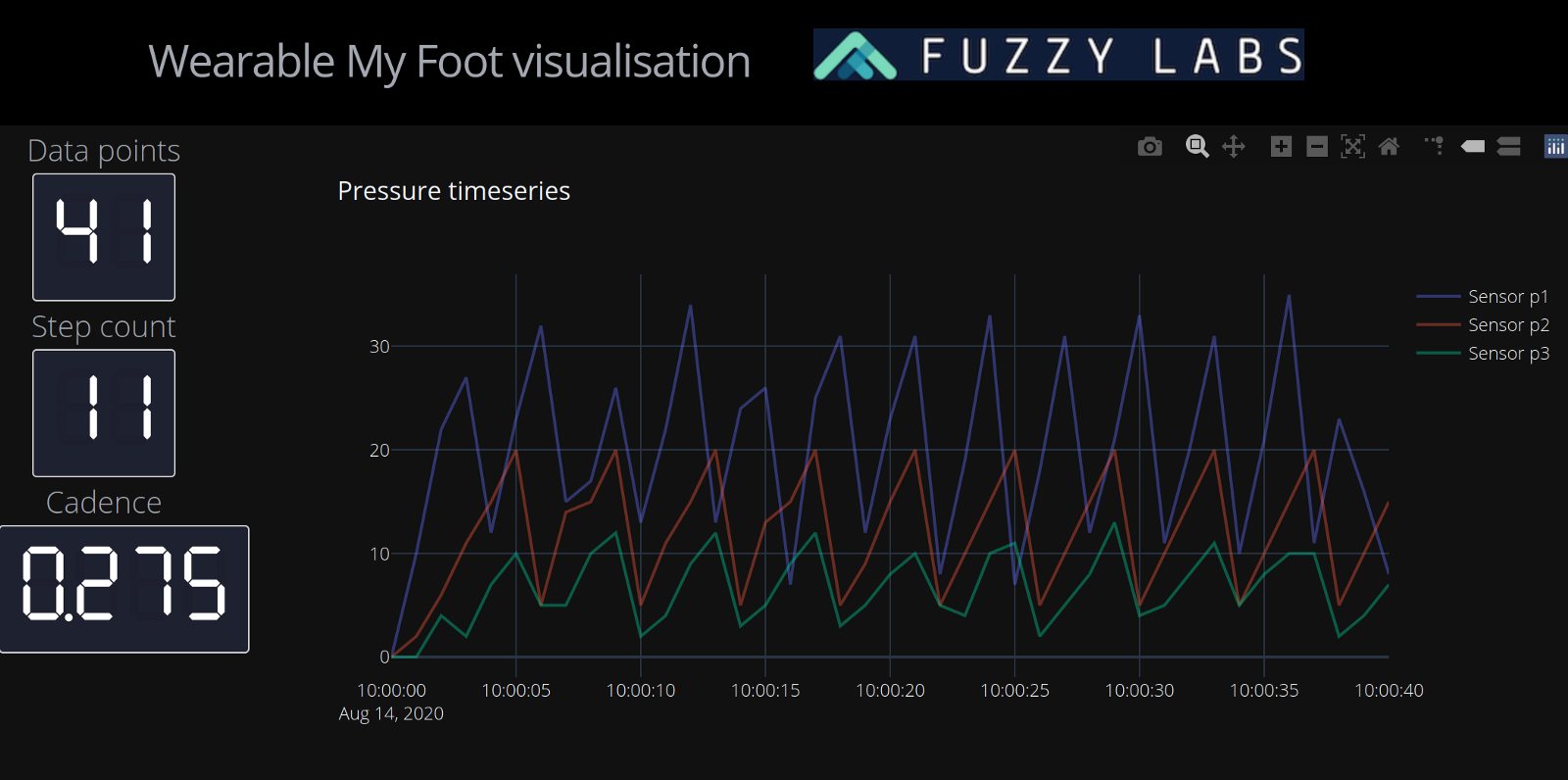
With Dash we can drop in the code that we already wrote in Jupyter. The only additional work is in laying out the dashboard and turning the graphs into Plotly graphs (instead of the matplotlib based graphs that Pandas generates).

As an example, here’s how we can turn our pressure sensor plot from earlier into a Plotly graph:

import plotly.graph_objs as go
pressure_plots = []
for sensor in ["p1", "p2", "p3"]:
    series = dataframe[sensor]
    scatter = go.Scatter(x = dataframe.index,
                         y = series,
                         name = f"Sensor {sensor}",
                         opacity = 0.4)
    pressure_plots.append(scatter)
pressure_figure = go.Figure(
    data = pressure_plots,
    layout = go.Layout(
        title = "Pressure timeseries"
    )
)

‍‍I’ll write a longer blog on the use of Dash, but here are a few important things to keep in mind when building dashboards:

• See the documentation for good examples of graphs and charts.
• Take a look at the Dash gallery for further inspiration.
• It’s a good idea to separate the logic for processing data and generating graphs from the setup and layout of the dashboard. For instance as three Python files: app.py, data_helper.py and graph_helper.py.
• Styling Dash can be a bit fiddly, but there’s a styleguide created by Chris P that simplifies this.

Contributing

We’re building open source tools for personalised fitness and healthcare devices and we’re keen for people to get involved in what we think is a pretty exciting area.

We’re grateful for the feedback we’ve received on social media, please keep it coming, and if you want to help out with hardware, software, data, design, or indeed testing some experimental devices, then let us know!