HuggingFace in Space 🤗 : Unlocking the Power of Pre-trained Embeddings with HuggingFace

Introduction

In a previous blog we discussed what embeddings are, how they are created and how we can use them in applications such as recommender systems. In this blog, we will discuss how to generate embeddings for a set of images using HuggingFace and PyTorch. 

You can follow along with the code in the notebook.

HuggingFace provides easy access to pre-trained models. Specifically, their ‘Transformers’ Python package provides APIs and tools to easily download and train state-of-the-art pre-trained models from the likes of Facebook and Google.

Pre-Trained Encoders with HuggingFace and PyTorch

Dataset

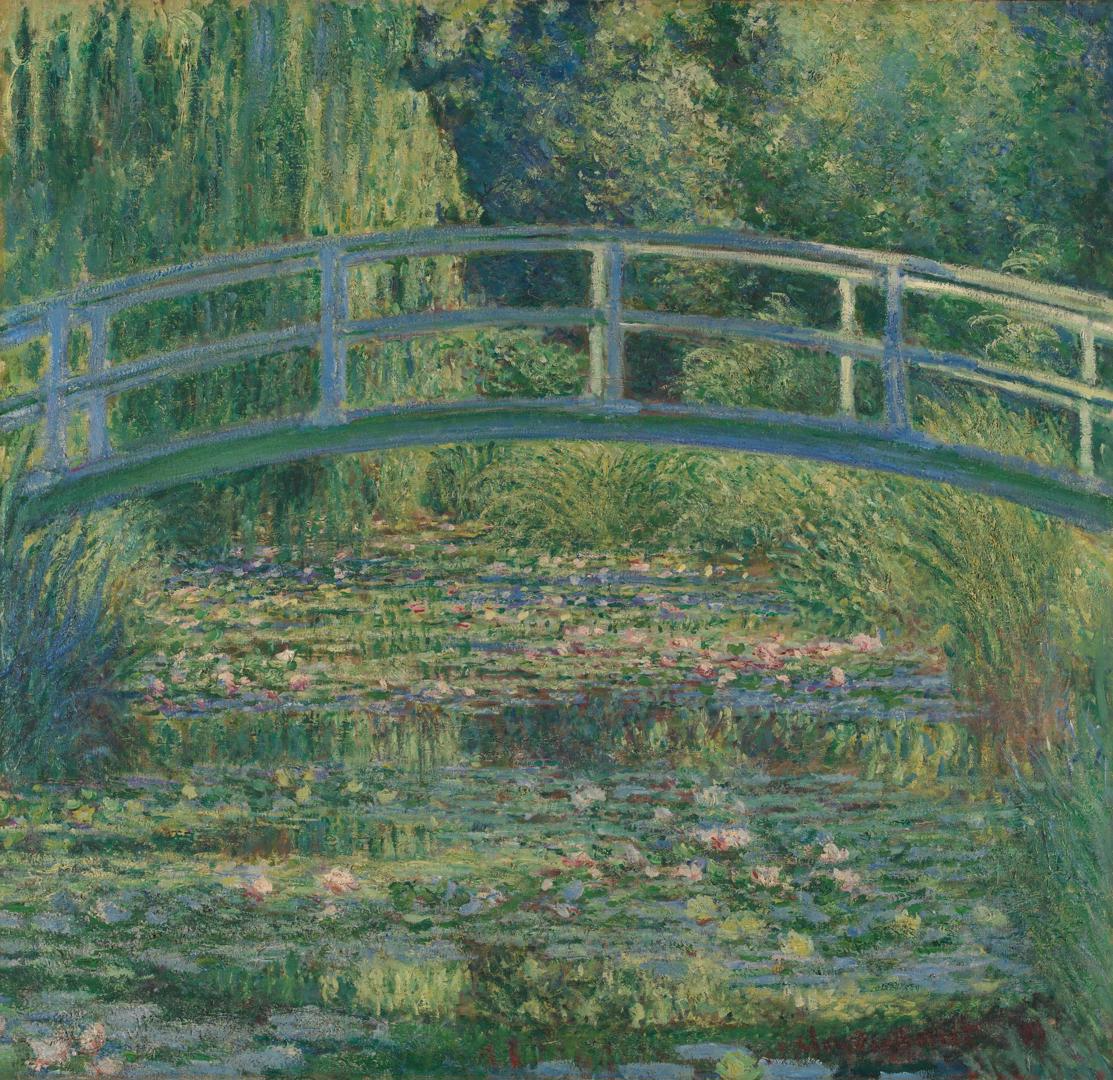
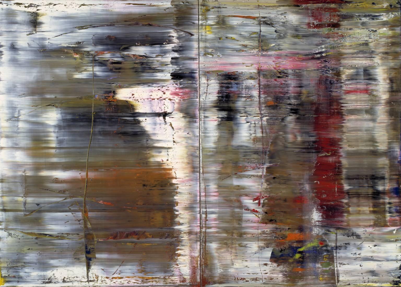
Before we get onto using the model we need to understand what data we want to create embeddings for. In our example, we will look at three artists Claude Monet, Gerhard Richter, and M. C. Escher and, as a control group, some pictures of animals. For each artist, we have two images of pieces of art. Images of animals are used as a control group to compare with the other pieces of art. This is because the pre-trained model we will use has not been trained on pieces of art but it has been partially trained on various animals. Hence we know these embeddings should be well-defined.

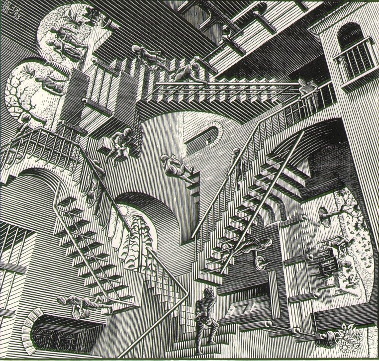
By visually inspecting our images, we can propose two hypotheses: 1) that each artwork will be grouped together by artists and 2) that artwork works which are visually similar will be grouped closer together (e.g., Monet's should be closer to Richters than Escher's based on their visual features). We will come back to these hypotheses later.

The structure of the data folder is as follows:<pre><code>data/
├── class1/
│   ├── image1.jpeg
│   └── image2.jpeg
├── class2/
│   ├── image3.jpeg
│   └── image4.jpeg
└── metadata.csv</pre></code>

Although for our example the class folders are not required it makes visualisation a bit easier. Within the metadata CSV, we list each file location and give it a corresponding shortened name so we can label the embeddings when it comes to visualisation.

HuggingFaces “datasets” package allows simple dataset creation using our data folder as follows:<pre><code>from datasets import load_dataset
image_dataset = load_dataset("imagefolder", data_dir="data/")

# Remove train/test segmentation
image_dataset = image_dataset['train']</pre></code

This stores the images in a HuggingFace dataset in Pillow (PIL) format.

The HuggingFace `load_dataset` function automatically puts all the data within a `train` set, for our example, we do not need a train and test dataset so we simply remove this for simplicity.

Following on from the previous blog we will be using HuggingFace's pre-trained version of the ViTMAE (Vision Transformers are Masked Auto-Encoders) model. This has been pre-trained on imagenet-1k which contains 14,197,122 images belonging to, as the name suggests, 1000 object classes. 

​​Using the two lines below, we initialize and download a pre-trained model named "facebook/vit-mae-base" and the corresponding image processor. <pre><code>from transformers import AutoImageProcessor, ViTMAEModel
model = ViTMAEModel.from_pretrained("facebook/vit-mae-base")image_processor = AutoImageProcessor.from_pretrained("facebook/vit-mae-base")</pre></code>

Image preprocessing

Once we have the model and image processor downloaded we can preprocess the images:<pre><code># Convert images to RGB if they are not already
image_dataset = image_dataset.map(lambda row: {"image": row['image'].convert("RGB")})
# Process images using HuggingFace processor
image_dataset = image_dataset.map(lambda row: {"preprocessed_image": image_processor(images=row['image'], return_tensors="pt")})

# Set dataset format to PyTorch
image_dataset = image_dataset.with_format("pt")</pre></code>

The code above transforms and splits the image up into sections called “tokens” which are required for the transformer architecture. We also convert all the PIL images into RGB which is required for the model. Finally, we set the dataset to use PyTorch tensors.

That’s it. All the components required to produce embeddings are now in place. So how do we produce embeddings?

Creating the image embeddings

<pre><code>def create_embedding(model: PreTrainedModel, preprocessed_image: torch.Tensor) -> torch.Tensor:
  """Passes a preprocessed image through a pretrained embedding model.

  Args:
      model (PreTrainedModel): Pretrained HuggingFace PyTorch embedding model.
      preprocessed_image (torch.Tensor): Preprocessed image as a PyTorch Tensor

  Returns:
      torch.Tensor: Embedding vector shape (1, 768) as a Tensor
  """
  embedding = model(**preprocessed_image).last_hidden_state[:, 0]
return np.squeeze(embedding) </pre></code>

The function above creates the embedding for a single preprocessed image. It takes the parameters of a HuggingFace pre-trained model and a pre-processed image tensor. The function passes this tensor into the model and extracts the values from the last hidden state. The slice `[:, 0]` is there to take the embedding value for a class token which is appended to the start of the token sequence for the image. This is a feature of ViT architecture (see the original paper Masked Autoencoders Are Scalable Vision Learners section “A. Implementation Details” for more information). An alternative way to extract embeddings is to (average) pool the last hidden states values to get the embedding vector:<pre><code>embedding = torch.mean(model(**preprocessed_image).last_hidden_state[:, 0], dim = 0)</pre></code>

In a production system, it would make more sense to pass the images to the model in batches to speed up the processing time. 

This function is then called within the dataset map function on each preprocessed image in the dataset.<pre><code>image_dataset = image_dataset.map(lambda img: {"embedding": create_embedding(model, img["preprocessed_image"])})</pre></code>Printing out the dataset shows the expected columns:<pre><code>Dataset({
    features: ['image', 'name', 'preprocessed_image', 'embedding'],
    num_rows: 9
})</pre></code>

We have successfully passed our images through the model and extracted the embeddings. 

Visualisation

Now that we have obtained a vector embedding for each image, how can we visualise where these lie in the embedding space? Doing this will allow us to objectively evaluate the embeddings. 

As visualising 700-800 dimensions is not feasible we need to use dimension reduction techniques to do this. Popular ways include Principal Component Analysis (PCA) and t-distributed stochastic neighbour embedding (T-SNE). 

For more information about these techniques visit 

PCA: https://royalsocietypublishing.org/doi/10.1098/rsta.2015.0202

T-SNE: https://distill.pub/2016/misread-tsne/

Luckily for us, TensorFlow has created an online tool (link here) that can perform these dimension reductions and plot them on an interactive 2D or 3D graph.

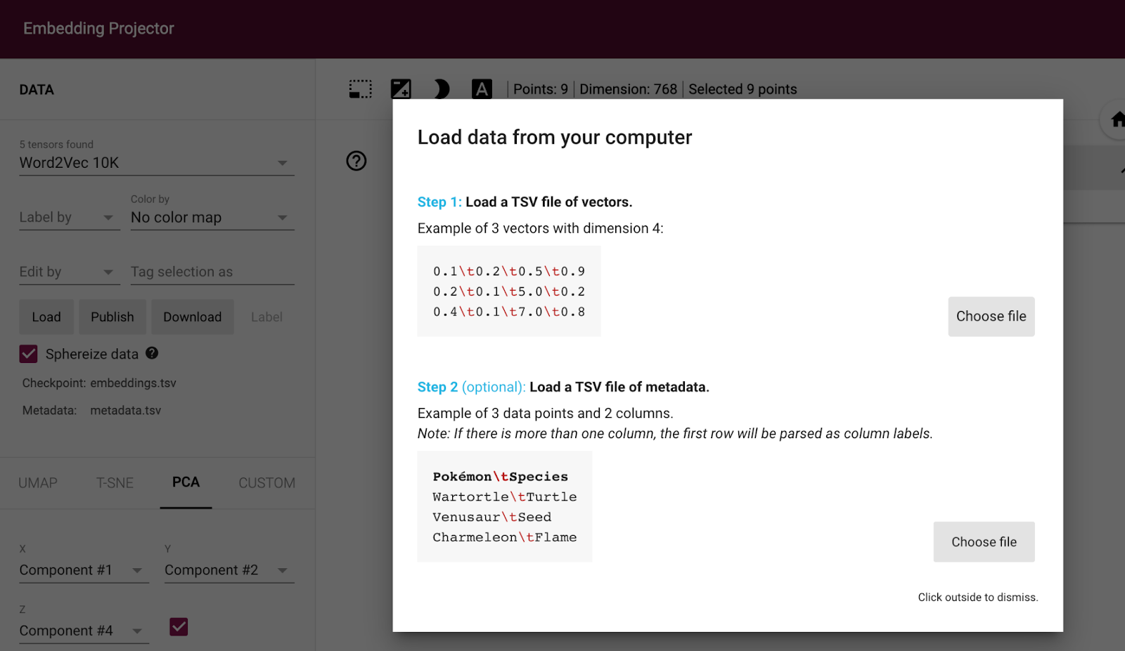
The data upload requires embeddings in a tab-separated value (TSV) file format. The notebook contains a method for producing two files, one containing the embedding vectors and the other containing the corresponding metadata required to display name labels.

‍

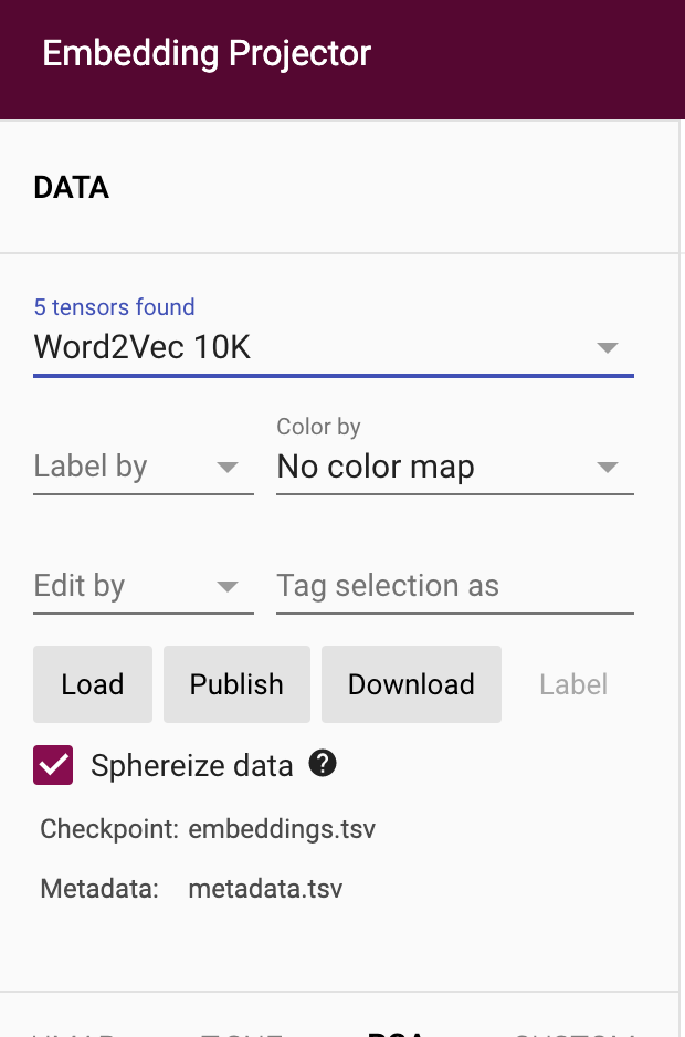
To upload data navigate to the column on the left-hand side of the screen and press “Load”. This will bring you to the following page where you can upload, first the `embeddings.tsv` file then the `metadata.tsv` file and then click outside the popup to visualise the embeddings. 

‍

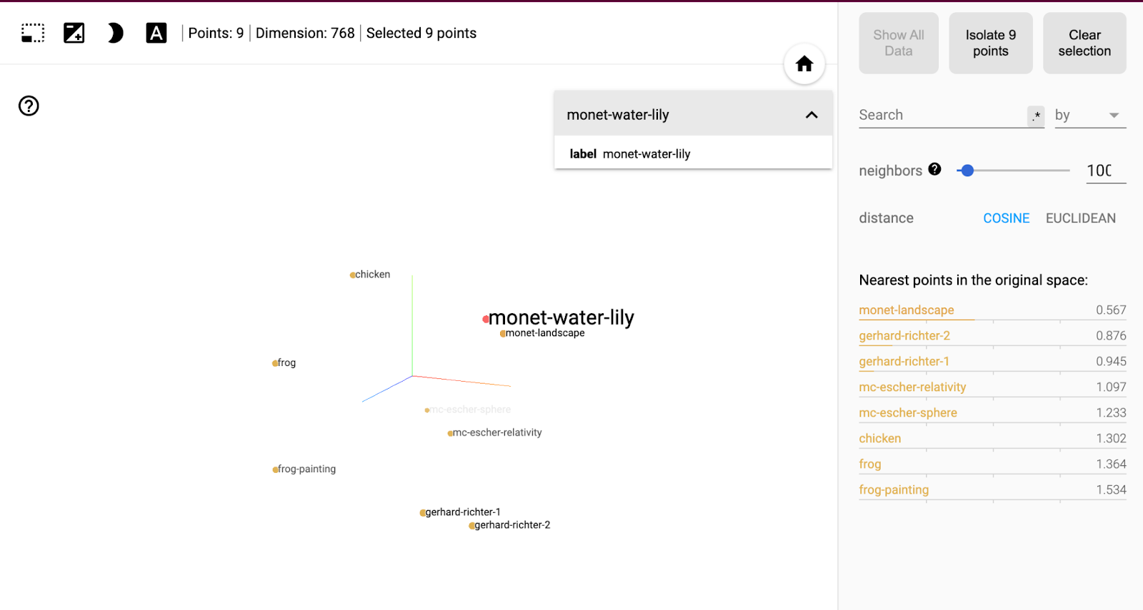
If we use PCA and select the “monet-water-lily” embedding we can see that the closest embeddings (using cosine distance) are the Monet landscape, followed by the Gerhard Richter paintings. The furthest away are the images of/depicting animals. This is roughly what we expected from our initial hypothesis.

Now that we have experimented with our embeddings how would we put these steps into production?

Machine Learning Operations (MLOps) for Embeddings

In the previous sections we have learned how to create embeddings and subjectively evaluated them. Two key concepts within MLOps workflows are especially valuable when working with embeddings in a production setting, these are data/machine learning pipelines and feature stores.

Data/Machine Learning Pipelines

Jupyter Notebooks are great for experimenting. In production, cracks can start to show and they are not built for huge amounts of data all stored in memory. This is where machine learning/feature pipelines come in. They are effectively a series of processing steps or statements which orchestrate the flow of data into, and output from, a machine learning model. Some advantages of using pipelines include

1. Reproducibility: Pipelines allow you to specify all the steps required to process your data, and you can save the configuration as a script or a file. This makes it easier to reproduce your analysis on new data or a different machine. In contrast, Jupyter Notebooks can be difficult to reproduce because they mix code, text, and output in a single document.
2. Scalability: Pipelines can be run on large datasets and leverage distributed computing systems like Spark or Hadoop. Jupyter Notebooks are not designed for large-scale data processing, and running them on large datasets can be slow and resource-intensive.
3. Debugging: Pipelines are easier to debug because each step in the pipeline is a separate function or module. You can test each step individually and isolate the source of errors more easily. In contrast, debugging Jupyter Notebooks can be challenging because of the interactivity and the mix of code and output.
4. Collaboration: Pipelines can be shared and reused more easily than Jupyter Notebooks. You can version control the code and the configuration files and share them with your colleagues or the community. In contrast, Jupyter Notebooks can be difficult to share and collaborate on because they mix code, text, and output in a single document, and the output may depend on the state of the kernel.

Some popular machine-learning pipeline tools include ZenML, Kubeflow, MLFlow and Kedro. 

Within the GitHub repository for this blog, we also provide a directory “zenml-pipeline” where we have converted our notebook code into a ZenML pipeline. See the instructions within the README on how to run this pipeline. For more information about ZenML pipelines see our blog here.

Feature Stores

The embeddings created will undoubtedly be used in downstream tasks such as recommender systems. In systems like these, fast access and queries of embeddings are essential.

‍

Feature stores are well-suited for storing embeddings because embeddings are typically high-dimensional vectors that represent complex relationships between data points. Here are some reasons why feature stores are good for storing embeddings:

‍

1. Efficient storage: Embeddings can be large and high-dimensional, making them computationally expensive to store and retrieve. A feature store can help optimise the storage and retrieval of embeddings by compressing them or storing them in a format that is optimised for fast retrievals, such as a vector database.

‍

2. Consistent feature management: Embeddings are often generated using complex machine learning models that can be difficult to reproduce. By storing embeddings in a feature store, we can ensure that the embeddings are consistently named, formatted, and stored, making it easier to manage and reuse them across different parts of the machine learning pipeline.

‍

3. Centralised feature management: Embeddings can be used for a wide range of machine learning tasks, from classification to clustering to recommendation systems. A feature store can provide a centralised repository for managing and serving embeddings, making it easier to share them across different teams and projects.

‍

4. Versioning and tracking: Embeddings are often generated using models that are refined over time with changing input data. By storing embeddings in a feature store, we can track the version history of each embedding and easily roll back to previous versions if necessary.

‍

5. Integration with model serving: Embeddings are often used as inputs to machine learning models for tasks such as classification or clustering. A feature store can provide an integration point for serving embeddings to models, making it easier to manage the dependencies between the embeddings and the models.

‍

Overall, using a feature store when creating embeddings can help improve the scalability, reproducibility, and maintainability of the machine learning pipeline. By providing a centralised repository for managing and sharing features, a feature store can help ensure that the embeddings are well-documented, consistent, and reusable across different downstream tasks. Some examples of open-source feature stores include Feast and Hopworks.

Optimising and Scaling Embedding Retrieval

Nearest neighbour search will suffice with 100 to 1000 embeddings but what happens when we scale this up to the millions or billions of embeddings? We can’t feasibly calculate the distance between every embedding in real-time with this sort of scale.

Alongside the use of MLOps tooling, there are several ways to optimise embedding retrieval. 

One example is using FAISS indexes: FAISS (Facebook AI Similarity Search) is an open-source library for fast similarity search on large-scale datasets with billions of embeddings.

At a very high level, FAISS indexes work by dividing the embedding space into multiple cells and storing the embeddings in each cell. During retrieval, the query embedding is compared to a subset of the embeddings in the index, based on the cells that are likely to contain the nearest neighbours. This reduces the number of embeddings that need to be compared, making the search more efficient. 

Adding FAISS indexes to HuggingFace datasets (more information here) is as easy as adding a single line of code:<pre><code>ds_with_embeddings.add_faiss_index(column='embeddings')</pre></code>

FAISS combines a number of techniques including:

1. Approximate nearest neighbour (ANN) search: ANN search is a technique for finding the nearest neighbours to a query point in a high-dimensional space. ANN search can be used to quickly identify embeddings that are similar to a given query, without computing the exact distance between every embedding in the dataset.

2. Quantization: By quantizing floating-point values in the embeddings to low-precision numbers that require fewer bits, embedding searches can be sped up and the embeddings will use less memory and space to store.

3. Index partitioning: Index partitioning involves splitting the dataset into multiple partitions or shards, each of which can be searched independently. This can improve the efficiency of similarity search by reducing the amount of data that needs to be processed in each query.

Overall, optimising embedding retrieval is critical for improving the performance and efficiency of machine learning applications. Techniques such as FAISS indexes, ANN search, dimensionality reduction, quantization, and index partitioning can all be used to improve the efficiency of embedding retrieval, depending on the specific use case and requirements.

Conclusion

In this blog we have shown you how to create powerful image embeddings using a pre-trained model from HuggingFace. We have also considered the potential risks when scaling this system in a production setting and how MLOps best practices and tools can help.

If you’d like to learn more about embeddings go to our other blog here.

‍

‍